3D computer graphics

Jump to: navigation, search

This article is about process of creating 3D computer graphics. For information on the study of computer graphics, see Computer graphics.

3D computer graphics

Basics
3D modeling / 3D scanning
3D rendering / 3D printing
3D computer graphics software
Primary Uses
3D models / Computer-aided design
Graphic design / Video games
Visual effects / Visualization
Virtual engineering / Virtual reality
Related concepts
CGI / Animation / 3D display
Wireframe model / Texture mapping
Computer animation / Motion capture
Skeletal animation / Crowd simulation
Global illumination / Volume rendering
This box: view • talk

3D computer graphics (in contrast to 2D computer graphics) are graphics that use a three-dimensional representation of geometric data (often Cartesian) that is stored in the computer for the purposes of performing calculations and rendering 2D images. Such images may be for later display or for real-time viewing.

Despite these differences, 3D computer graphics rely on many of the same algorithms as 2D computer vector graphics in the wire-frame model and 2D computer raster graphics in the final rendered display. In computer graphics software, the distinction between 2D and 3D is occasionally blurred; 2D applications may use 3D techniques to achieve effects such as lighting, and primarily 3D may use 2D rendering techniques.

3D computer graphics are often referred to as 3D models. Apart from the rendered graphic, the model is contained within the graphical data file. However, there are differences. A 3D model is the mathematical representation of any three-dimensional object (either inanimate or living). A model is not technically a graphic until it is visually displayed. Due to 3D printing, 3D models are not confined to virtual space. A model can be displayed visually as a two-dimensional image through a process called 3D rendering, or used in non-graphical computer simulations and calculations.

Contents [hide] 1 History 2 Overview 2.1 Modeling 2.2 Layout and animation 2.3 Rendering 3 Communities 4 Distinction from photorealistic 2D graphics 5 See also 6 References 7 External links

[edit] History

William Fetter was credited with coining the term computer graphics in 1960^[1][2], to describe his work at Boeing. One of the first displays of computer animation was Futureworld (1976), which included an animation of a human face and hand — produced by Ed Catmull and Fred Parke at the University of Utah.

[edit] Overview

The process of creating 3D computer graphics can be sequentially divided into three basic phases: 3D modeling which describes the process of forming the shape of an object, layout and animation which describes the motion and placement of objects within a scene, and 3D rendering which produces an image of an object.

[edit] Modeling

A 3D rendering with ray tracing and ambient occlusion using Blender and Yafray

Main article: 3D modeling

The model describes the process of forming the shape of an object. The two most common sources of 3D models are those originated on the computer by an artist or engineer using some kind of 3D modeling tool, and those scanned into a computer from real-world objects. Models can also be produced procedurally or via physical simulation.

[edit] Layout and animation

Main article: Computer animation

Before objects are rendered, they must be placed (laid out) within a scene. This is what defines the spatial relationships between objects in a scene including location and size. Animation refers to the temporal description of an object, i.e., how it moves and deforms over time. Popular methods include keyframing, inverse kinematics, and motion capture, though many of these techniques are used in conjunction with each other. As with modeling, physical simulation is another way of specifying motion.

[edit] Rendering

During the 3D rendering step, the number of reflections “light rays” can take, as well as various other attributes, can be tailored to achieve a desired visual effect.

Main article: 3D rendering

Rendering converts a model into an image either by simulating light transport to get photorealistic images, or by applying some kind of style as in non-photorealistic rendering. The two basic operations in realistic rendering are transport (how much light gets from one place to another) and scattering (how surfaces interact with light). This step is usually performed using 3D computer graphics software or a 3D graphics API. The process of altering the scene into a suitable form for rendering also involves 3D projection which allows a three-dimensional image to be viewed in two dimensions.

[edit] Communities

There are a multitude of websites designed to help educate and support 3D graphic artists. Some are managed by software developers and content providers, but there are standalone sites as well. These communities allow for members to seek advice, post tutorials, provide product reviews or post examples of their own work.

[edit] Distinction from photorealistic 2D graphics

Not all computer graphics that appear 3D are based on a wireframe model. 2D computer graphics with 3D photorealistic effects are often achieved without wireframe modeling and are sometimes indistinguishable in the final form. Some graphic art software includes filters that can be applied to 2D vector graphics or 2D raster graphics on transparent layers. Visual artists may also copy or visualize 3D effects and manually render photorealistic effects without the use of filters. See also still life.^{[citation needed]}

[edit] See also

• 3D computer graphics software
• 3D motion controller
• 3D projection on 2D planes
• Anaglyph image
• Computer vision
• Digital geometry
• Geometry pipeline
• Geometry processing
• Graphics
• Graphics processing unit (GPU)
• Graphical output devices
• Image processing
• Reflection (computer graphics)
• Rendering (computer graphics)
• SIGGRAPH
• Timeline of CGI in films
• Computer-animated television series

[edit] References

1. ^ An Historical Timeline of Computer Graphics and Animation
2. ^ Computer Graphics, comphist.org

Visual analytics

Jump to: navigation, search

Scalable Reasoning Systems: Technology to support knowledge transfer and cooperative inquiry must offer its users the ability to effectively interpret knowledge structures produced by collaborators.^[1]

Visual analytics is an outgrowth of the fields information visualization and scientific visualization, that focuses on analytical reasoning facilitated by interactive visual interfaces.^[2]

Contents [hide] 1 Overview 2 Topics 2.1 Scope 2.2 Analytical reasoning techniques 2.3 Data representations 2.4 Theories of visualization 2.5 Visual representations 3 Process 4 See also 5 References 6 Further reading 7 External links

[edit] Overview

Visual analytics is "the integration of interactive visualization with analysis techniques to answer a growing range of questions in science, business, and analysis. It can attack certain problems whose size, complexity, and need for closely coupled human and machine analysis may make them otherwise intractable. Visual analytics encompasses topics in computer graphics, interaction, visualization, analytics, perception, and cognition".^[3]

R&D for Visual Analytics.

Visual analytics integrates new computational and theory-based tools with innovative interactive techniques and visual representations to enable human-information discourse. The design of the tools and techniques is based on cognitive, design, and perceptual principles. This science of analytical reasoning provides the reasoning framework upon which one can build both strategic and tactical visual analytics technologies for threat analysis, prevention, and response. Analytical reasoning is central to the analyst’s task of applying human judgments to reach conclusions from a combination of evidence and assumptions.^[4]

Visual analytics has some overlapping goals and techniques with information visualization and scientific visualization. There is currently no clear consensus on the boundaries between these fields, but broadly speaking the three areas can be distinguished as follows. Scientific visualization deals with data that has a natural geometric structure (e.g., MRI data, wind flows). Information visualization handles abstract data structures such as trees or graphs. Visual analytics is especially concerned with sensemaking and reasoning.

Visual analytics seeks to marry techniques from information visualization with techniques from computational transformation and analysis of data. Information visualization itself forms part of the direct interface between user and machine. Information visualization amplifies human cognitive capabilities in six basic ways:^{[4] [5]}

1. by increasing cognitive resources, such as by using a visual resource to expand human working memory,
2. by reducing search, such as by representing a large amount of data in a small space,
3. by enhancing the recognition of patterns, such as when information is organized in space by its time relationships,
4. by supporting the easy perceptual inference of relationships that are otherwise more difficult to induce,
5. by perceptual monitoring of a large number of potential events, and
6. by providing a manipulable medium that, unlike static diagrams, enables the exploration of a space of parameter values.

These capabilities of information visualization, combined with computational data analysis, can be applied to analytic reasoning to support the sense-making process.

[edit] Topics

[edit] Scope

Visual analytics: research and practice.^[6]

Visual analytics is a multidisciplinary field that includes the following focus areas:^[4]

• Analytical reasoning techniques that enable users to obtain deep insights that directly support assessment, planning, and decision making
• Data representations and transformations that convert all types of conflicting and dynamic data in ways that support visualization and analysis
• Techniques to support production, presentation, and dissemination of the results of an analysis to communicate information in the appropriate context to a variety of audiences.
• Visual representations and interaction techniques that take advantage of the human eye’s broad bandwidth pathway into the mind to allow users to see, explore, and understand large amounts of information at once

[edit] Analytical reasoning techniques

Analytical reasoning techniques are the method by which users obtain deep insights that directly support situation assessment, planning, and decision making. Visual analytics must facilitate high-quality human judgment with a limited investment of the analysts’ time. Visual analytics tools must enable diverse analytical tasks such as:^[4]

• Understanding past and present situations quickly, as well as the trends and events that have produced current conditions
• Identifying possible alternative futures and their warning signs
• Monitoring current events for emergence of warning signs as well as unexpected events
• Determining indicators of the intent of an action or an individual
• Supporting the decision maker in times of crisis.

These tasks will be conducted through a combination of individual and collaborative analysis, often under extreme time pressure. Visual analytics must enable hypothesis-based and scenario-based analytical techniques, providing support for the analyst to reason based on the available evidence.^[4]

[edit] Data representations

Data representations are structured forms suitable for computer-based transformations. These structures must exist in the original data or be derivable from the data themselves. They must retain the information and knowledge content and the related context within the original data to the greatest degree possible. The structures of underlying data representations are generally neither accessible nor intuitive to the user of the visual analytics tool. They are frequently more complex in nature than the original data and are not necessarily smaller in size than the original data. The structures of the data representations may contain hundreds or thousands of dimensions and be unintelligible to a person, but they must be transformable into lower-dimensional representations for visualization and analysis.^[4]

[edit] Theories of visualization

Theories of visualization are:^[3]

• "Semiology of Graphics" in 1967 written by Jacques Bertin e
• "Languages of Art" from 1977 by Nelson Goodman
• Jock D. Mackinlay's "Automated design of optimal visualization" (APT) from 1986, and
• Leland Wilkinson's "Grammar of Graphics" from 1998,

[edit] Visual representations

Visual representations translate data into a visible form that highlights important features, including commonalities and anomalies. These visual representations make it easy for users to perceive salient aspects of their data quickly. Augmenting the cognitive reasoning process with perceptual reasoning through visual representations permits the analytical reasoning process to become faster and more focused.^[4]

[edit] Process

The input for the data sets used in the visual analytics process are heterogeneous data sources (i.e., the internet, newspapers, books, scientific experiments, expert systems). From these rich sources, the data sets S = S₁, ..., S_m are chosen, whereas each S_i , i ∈ (1, ..., m) consists of attributes A_i1, ..., A_ik. The goal or output of the process is insight I. Insight is either directly obtained from the set of created visualizations V or through confirmation of hypotheses H as the results of automated analysis methods. This formalization of the visual analytics process is illustrated in the following figure. Arrows represent the transitions from one set to another one.

More formal the visual analytics process is a transformation F : S → I, whereas F is a concatenation of functions f ∈ {D_W, V_X, H_Y, U_Z} defined as follows:

D_W describes the basic data pre-processing functionality with D_W : S → S and W ∈ {T, C, SL, I} including data transformation functions D_T, data cleaning functions D_C, data selection functions D_SL and data integration functions D_I that are needed to make analysis functions applicable to the data set.

V_W, W ∈ {S, H} symbolizes the visualization functions, which are either functions visualizing data V_S : S → V or functions visualizing hypotheses V_H : H → V.

H_Y, Y ∈ {S, V} represents the hypotheses generation process. We distinguish between functions that generate hyphotheses from data H_S : S → H and functions that generate hypotheses from visualizations H_V : V → H.

Moreover, user interactions U_Z, Z ∈ {V, H, CV, CH} are an integral part of the visual analytics process. User interactions can either effect only visualizations U_V : V → V (i.e., selecting or zooming), or can effect only hypotheses U_H : H → H by generating a new hypotheses from given ones. Furthermore, insight can be concluded from visualizations U_CV : V → I or from hypotheses U_CH : H → I.

The typical data pre-processing applying data cleaning, data integration and data transformation functions is defined as D_P = D_T(D_I(D_C(S₁, ..., S_n))). After the pre-processing step either automated analysis methods H_S = {f_s1, ..., f_sq} (i.e., statistics, data mining, etc.) or visualization methods V_S : S → V, V_S = {f_v1, ..., f_vs} are applied to the data, in order to reveal patterns as shown in the figure above.^[7]

[edit] See also

An application: Intelligent Multi-Agent System for Knowledge discovery. Researchers are working on the design and development of systems that enhance human-information interaction in information analysis and discovery for diverse applications, such as intelligence analysis and bio-informatics.^[1]

Related subjects

• Argument mapping
• Business Decision Mapping
• Computational visualistics
• Critical thinking
• Decision making
• Diagrammatic reasoning
• Geovisualization
• Google Analytics
• Social network analysis software
• Software visualization
• Starlight Information Visualization System
• Text analytics
• Traffic analysis
• Visual reasoning
• Wicked problem

Related scientists

• Cecilia R. Aragon
• Robert E. Horn
• Daniel A. Keim
• Theresa-Marie Rhyne
• Lawrence J. Rosenblum
• John Stasko

[edit] References

1. ^ ^{a b} Pacific Northwest National Laboratory (PNNL) Cognitive Informatics research and development in human information interaction. Retrieved 1 July 2008.
2. ^ Pak Chung Wong and J. Thomas (2004). "Visual Analytics". in: IEEE Computer Graphics and Applications, Volume 24, Issue 5, Sept.-Oct. 2004 Page(s): 20–21.
3. ^ ^{a b} Robert Kosara (2007). Visual Analytics. ITCS 4122/5122, Fall 2007. Retrieved 28 june 2008.
4. ^ ^{a b c d e f g} James J. Thomas and Kristin A. Cook (Ed.) (2005). Illuminating the Path: The R&D Agenda for Visual Analytics. National Visualization and Analytics Center. p.3–33.
5. ^ Stuart Card, J.D. Mackinlay, and Ben Shneiderman (1999). "Readings in Information Visualization: Using Vision to Think". Morgan Kaufmann Publishers, San Francisco.
6. ^ National Visualization and Analytics Center. Retrieved 1 July 2008.
7. ^ Daniel A. Keim, Florian Mansmann, Jörn Schneidewind, Jim Thomas, and Hartmut Ziegler (2008). "Visual Analytics: Scope and Challenges"

[edit] Further reading

• Boris Kovalerchuk and James Schwing (2004). Visual and Spatial Analysis: Advances in Data Mining, Reasoning, and Problem Soving
• Guoping Qiu (2007). Advances in Visual Information Systems: 9th International Conference (VISUAL).
• IEEE, Inc. Staff (2007). Visual Analytics Science and Technology (VAST), A Symposium of the IEEE 2007.
• May Yuan, Kathleen and Stewart Hornsby (2007). Computation and Visualization for Understanding Dynamics in Geographic Domains.

[edit] External links

Wikimedia Commons has media related to: Visual analytics

• VisMaster Visual Analytics – Mastering the Information Age
• SPP - Scalable Visual Analytics
• Visual Analytics a course by Robert Kosara, 2007.
• IEEE Visual Analytics Science and Technology (VAST) Symposium
• National Visualization and Analytics Center (NVAC)
• Visual Analytics Digital Library (VADL)
• GeoAnalytics.net - GeoSpatial Visual Analytics, ICA commission

Spatial analysis

Map by Dr. John Snow of London, showing clusters of cholera cases in the 1854 Broad Street cholera outbreak. This was one of the first uses of map-based spatial analysis.

In statistics, spatial analysis or spatial statistics includes any of the formal techniques which study entities using their topological, geometric, or geographic properties. The phrase properly refers to a variety of techniques, many still in their early development, using different analytic approaches and applied in fields as diverse as astronomy, with its studies of the placement of galaxies in the cosmos, to chip fabrication engineering, with its use of 'place and route' algorithms to build complex wiring structures. The phrase is often used in a more restricted sense to describe techniques applied to structures at the human scale, most notably in the analysis of geographic data. The phrase is even sometimes used to refer to a specific technique in a single area of research, for example, to describe geostatistics.

The history of spatial analysis starts with early mapping, surveying and geography at the beginning of history, although the techniques of spatial analysis were not formalized until the later part of the twentieth century. Modern spatial analysis focuses on computer based techniques because of the large amount of data, the power of modern statistical and geographic information science (GIS) software, and the complexity of the computational modeling. Spatial analytic techniques have been developed in geography, biology, epidemiology, sociology, demography, statistics, geographic information science, remote sensing, computer science, mathematics, and scientific modelling.

Complex issues arise in spatial analysis, many of which are neither clearly defined nor completely resolved, but form the basis for current research. The most fundamental of these is the problem of defining the spatial location of the entities being studied. For example, a study on human health could describe the spatial position of humans with a point placed where they live, or with a point located where they work, or by using a line to describe their weekly trips; each choice has dramatic effects on the techniques which can be used for the analysis and on the conclusions which can be obtained. Other issues in spatial analysis include the limitations of mathematical knowledge, the assumptions required by existing statistical techniques, and problems in computer based calculations.

Classification of the techniques of spatial analysis is difficult because of the large number of different fields of research involved, the different fundamental approaches which can be chosen, and the many forms the data can take.

Contents [hide] 1 The history of spatial analysis 2 Fundamental issues in spatial analysis 2.1 Spatial characterization 2.2 Spatial dependency or auto-correlation 2.3 Scaling 2.4 Sampling 2.5 Common errors in spatial analysis 2.5.1 Length 2.5.2 Locational fallacy 2.5.3 Atomic fallacy 2.5.4 Ecological fallacy 2.5.5 Modifiable areal unit problem 2.6 Solutions to the fundamental issues 2.6.1 Geographic space 3 Types of spatial analysis 3.1 Spatial autocorrelation 3.2 Spatial interpolation 3.3 Spatial regression 3.4 Spatial interaction 3.5 Simulation and modeling 4 Geographic information science and spatial analysis 5 See also 6 References 7 Further reading 8 External links

[edit] The history of spatial analysis

Spatial analysis can perhaps be considered to have arisen with the early attempts at cartography and surveying but many fields have contributed to its rise in modern form. Biology contributed through botanical studies of global plant distributions and local plant locations, ethological studies of animal movement, landscape ecological studies of vegetation blocks, ecological studies of spatial population dynamics, and the study of biogeography. Epidemiology contributed with early work on disease mapping, notably John Snow's work mapping an outbreak of cholera, with research on mapping the spread of disease and with locational studies for health care delivery. Statistics has contributed greatly through work in spatial statistics. Economics has contributed notably through spatial econometrics. Geographic information system is currently a major contributor due to the importance of geographic software in the modern analytic toolbox. Remote sensing has contributed extensively in morphometric and clustering analysis. Computer science has contributed extensively through the study of algorithms, notably in computational geometry. Mathematics continues to provide the fundamental tools for analysis and to reveal the complexity of the spatial realm, for example, with recent work on fractals and scale invariance. Scientific modelling provides a useful framework for new approaches.

[edit] Fundamental issues in spatial analysis

Spatial analysis confronts many fundamental issues in the definition of its objects of study, in the construction of the analytic operations to be used, in the use of computers for analysis, in the limitations and particularities of the analyses which are known, and in the presentation of analytic results. Many of these issues are active subjects of modern research.

Common errors often arise in spatial analysis, some due to the mathematics of space, some due to the particular ways data are presented spatially, some due to the tools which are available. Census data, because it protects individual privacy by aggregating data into local units, raises a number of statistical issues. Computer software can easily calculate the lengths of the lines which it defines but these may have no inherent meaning in the real world, as was shown for the coastline of Britain.

These problems represent one of the greatest dangers in spatial analysis because of the inherent power of maps as media of presentation. When results are presented as maps, the presentation combines the spatial data which is generally very accurate with analytic results which may be grossly inaccurate. Some of these issues are discussed at length in the book How to Lie with Maps^[1]

[edit] Spatial characterization

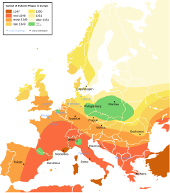
Spread of bubonic plague in medieval Europe. The colors indicate the spatial distribution of plague outbreaks over time. Possibly due to the limitations of printing or for a host of other reasons, the cartographer selected a discrete number of colors to characterize (and simplify) reality.

The definition of the spatial presence of an entity constrains the possible analysis which can be applied to that entity and influences the final conclusions that can be reached. While this property is fundamentally true of all analysis, it is particularly important in spatial analysis because the tools to define and study entities favor specific characterizations of the entities being studied. Statistical techniques favor the spatial definition of objects as points because there are very few statistical techniques which operate directly on line, area, or volume elements. Computer tools favor the spatial definition of objects as homogeneous and separate elements because of the primitive nature of the computational structures available and the ease with which these primitive structures can be created.

There may also be arbitrary effects introduced by the spatial bounds or limits placed on the phenomenon or study area. This occurs since spatial phenomena may be unbounded or have ambiguous transition zones. This creates edge effects from ignoring spatial dependency or interaction outside the study area. It also imposes artificial shapes on the study area that can affect apparent spatial patterns such as the degree of clustering. A possible solution is similar to the sensitivity analysis strategy for the modifiable areal unit problem, or MAUP: change the limits of the study area and compare the results of the analysis under each realization. Another possible solution is to overbound the study area. It is also feasible to eliminate edge effects in spatial modeling and simulation by mapping the region to a boundless object such as a torus or sphere.

[edit] Spatial dependency or auto-correlation

A fundamental concept in geography is that nearby entities often share more similarities than entities which are far apart. This idea is often labeled 'Tobler's first law of geography' and may be summarized as "everything is related to everything else, but near things are more related than distant things" ^[2].

Spatial dependency is the co-variation of properties within geographic space: characteristics at proximal locations appear to be correlated, either positively or negatively. There are at least three possible explanations. One possibility is there is a simple spatial correlation relationship: whatever is causing an observation in one location also causes similar observations in nearby locations. For example, physical crime rates in nearby areas within a city tend to be similar due to factors such as socio-economic status, amount of policing and the built environment creating the opportunities for that kind of crime: the features that attract one criminal will also attract others. Another possibility is spatial causality: something at a given location directly influences the characteristics of nearby locations. For example, the broken window theory of personal crime suggests that poverty, lack of maintenance and petty physical crime tends to breed more crime of this kind due to the apparent breakdown in order. A third possibility is spatial interaction: the movement of people, goods or information creates apparent relationships between locations. The “journey to crime” theory suggests that criminal activity occurs as a result of accessibility to a criminal’s home, hangout or other key locations in his or her daily activities.

Spatial dependency leads to the spatial autocorrelation problem in statistics since, like temporal autocorrelation, this violates standard statistical techniques that assume independence among observations. For example, regression analyses that do not compensate for spatial dependency can have unstable parameter estimates and yield unreliable significance tests. Spatial regression models (see below) capture these relationships and do not suffer from these weaknesses. It is also appropriate to view spatial dependency as a source of information rather than something to be corrected.

Locational effects also manifest as spatial heterogeneity, or the apparent variation in a process with respect to location in geographic space. Unless a space is uniform and boundless, every location will have some degree of uniqueness relative to the other locations. This affects the spatial dependency relations and therefore the spatial process. Spatial heterogeneity means that overall parameters estimated for the entire system may not adequately describe the process at any given location.

[edit] Scaling

Spatial scale is a persistent issue in spatial analysis.

One of these issues is a simple issue of language. Different fields use "large scale" and "small scale" to mean the opposite things, for example, cartographers referring to the mathematical size of the scale ratio, 1/24000 being 'larger' than 1/100000, while landscape ecologists long referred to the extent of their study areas, with continents being 'larger' than forests.

The more fundamental issue of scale requires ensuring that the conclusion of the analysis does not depend on any arbitrary scale. Landscape ecologists failed to do this for many years and for a long time characterized landscape elements with quantitative metrics which depended on the scale at which they were measured. They eventually developed a series of scale invariant metrics.

[edit] Sampling

Spatial sampling involves determining a limited number of locations in geographic space for faithfully measuring phenomena that are subject to dependency and heterogeneity. Dependency suggests that since one location can predict the value of another location, we do not need observations in both places. But heterogeneity suggests that this relation can change across space, and therefore we cannot trust an observed degree of dependency beyond a region that may be small. Basic spatial sampling schemes include random, clustered and systematic. These basic schemes can be applied at multiple levels in a designated spatial hierarchy (e.g., urban area, city, neighborhood). It is also possible to exploit ancillary data, for example, using property values as a guide in a spatial sampling scheme to measure educational attainment and income. Spatial models such as autocorrelation statistics, regression and interpolation (see below) can also dictate sample design.

[edit] Common errors in spatial analysis

The fundamental issues in spatial analysis lead to numerous problems in analysis including bias, distortion and outright errors in the conclusions reached. These issues are often interlinked but various attempts have been made to separate out particular issues from each other.

[edit] Length

In a paper by Benoit Mandelbrot on the coastline of Britain it was shown that it is inherently nonsensical to discuss certain spatial concepts despite an inherent presumption of the validity of the concept. Lengths in ecology depend directly on the scale at which they are measured and experienced. So while surveyors commonly measure the length of a river, this length only has meaning in the context of the relevance of the measuring technique to the question under study.

Britain measured using a long yardstick

Britain measured using a medium yardstick

Britain measured using a short yardstick

[edit] Locational fallacy

The locational fallacy refers to error due to the particular spatial characterization chosen for the elements of study, in particular choice of placement for the spatial presence of the element.

Spatial characterizations may be simplistic or even wrong. Studies of humans often reduce the spatial existence of humans to a single point, for instance their home address. This can easily lead to poor analysis, for example, when considering disease transmission which can happen at work or at school and therefore far from the home.

The spatial characterization may implicitly limit the subject of study. For example, the spatial analysis of crime data has recently become popular but these studies can only describe the particular kinds of crime which can be described spatially. This leads to many maps of assault but not to any maps of embezzlement with political consequences in the conceptualization of crime and the design of policies to address the issue.

[edit] Atomic fallacy

This describes errors due to treating elements as separate 'atoms' outside of their spatial context.

[edit] Ecological fallacy

The ecological fallacy describes errors due to performing analyses on aggregate data when trying to reach conclusions on the individual units. It is closely related to the modifiable areal unit problem.

[edit] Modifiable areal unit problem

The modifiable areal unit problem (MAUP) is an issue in the analysis of spatial data arranged in zones, where the conclusion depends on the particular shape or size of the zones used in the analysis.

Spatial analysis and modeling often involves aggregate spatial units such as census tracts or traffic analysis zones. These units may reflect data collection and/or modeling convenience rather than homogeneous, cohesive regions in the real world. The spatial units are therefore arbitrary or modifiable and contain artifacts related to the degree of spatial aggregation or the placement of boundaries.

The problem arises because it is known that results derived from an analysis of these zones depends directly on the zones being studied. It has been shown that the aggregation of point data into zones of different shapes and sizes can lead to opposite conclusions.^[3] More detail is available at the modifiable areal unit problem topic entry.

[edit] Solutions to the fundamental issues

[edit] Geographic space

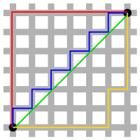
Manhattan distance versus Euclidean distance: The red, blue, and yellow lines have the same length (12) in both Euclidean and taxicab geometry. In Euclidean geometry, the green line has length 6×√2 ≈ 8.48, and is the unique shortest path. In taxicab geometry, the green line's length is still 12, making it no shorter than any other path shown.

A mathematical space exists whenever we have a set of observations and quantitative measures of their attributes. For example, we can represent individuals’ income or years of education within a coordinate system where the location of each individual can be specified with respect to both dimensions. The distances between individuals within this space is a quantitative measure of their differences with respect to income and education. However, in spatial analysis we are concerned with specific types of mathematical spaces, namely, geographic space. In geographic space, the observations correspond to locations in a spatial measurement framework that captures their proximity in the real world. The locations in a spatial measurement framework often represent locations on the surface of the Earth, but this is not strictly necessary. A spatial measurement framework can also capture proximity with respect to, say, interstellar space or within a biological entity such as a liver. The fundamental tenet is Tobler’s First Law of Geography: if the interrelation between entities increases with proximity in the real world, then representation in geographic space and assessment using spatial analysis techniques are appropriate.

The Euclidean distance between locations often represents their proximity, although this is only one possibility. There are an infinite number of distances in addition to Euclidean that can support quantitative analysis. For example, "Manhattan" (or "Taxicab") distances where movement is restricted to paths parallel to the axes can be more meaningful than Euclidean distances in urban settings. In addition to distances, other geographic relationships such as connectivity (e.g., the existence or degree of shared borders) and direction can also influence the relationships among entities. It is also possible to compute minimal cost paths across a cost surface; for example, this can represent proximity among locations when travel must occur across rugged terrain.

[edit] Types of spatial analysis

Spatial data comes in many varieties and it is not easy to arrive at a system of classification that is simultaneously exclusive, exhaustive, imaginative, and satisfying. -- G. Upton & B. Fingelton^[4]

[edit] Spatial autocorrelation

Spatial autocorrelation statistics measure and analyze the degree of dependency among observations in a geographic space. Classic spatial autocorrelation statistics include Moran’s I and Geary’s C. These require measuring a spatial weights matrix that reflects the intensity of the geographic relationship between observations in a neighborhood, e.g., the distances between neighbors, the lengths of shared border, or whether they fall into a specified directional class such as “west.” Classic spatial autocorrelation statistics compare the spatial weights to the covariance relationship at pairs of locations. Spatial autocorrelation that is more positive than expected from random indicate the clustering of similar values across geographic space, while significant negative spatial autocorrelation indicates that neighboring values are more dissimilar than expected by chance, suggesting a spatial pattern similar to a chess board.

Spatial autocorrelation statistics such as Moran’s I and Geary’s C are global in the sense that they estimate the overall degree of spatial autocorrelation for a dataset. The possibility of spatial heterogeneity suggests that the estimated degree of autocorrelation may vary significantly across geographic space. Local spatial autocorrelation statistics provide estimates disaggregated to the level of the spatial analysis units, allowing assessment of the dependency relationships across space. G statistics compare neighborhoods to a global average and identify local regions of strong autocorrelation. Local versions of the I and C statistics are also available.

[edit] Spatial interpolation

Spatial interpolation methods estimate the variables at unobserved locations in geographic space based on the values at observed locations. Basic methods include inverse distance weighting: this attenuates the variable with decreasing proximity from the observed location. Kriging is a more sophisticated method that interpolates across space according to a spatial lag relationship that has both systematic and random components. This can accommodate a wide range of spatial relationships for the hidden values between observed locations. Kriging provides optimal estimates given the hypothesized lag relationship, and error estimates can be mapped to determine if spatial patterns exist.

[edit] Spatial regression

Spatial regression methods capture spatial dependency in regression analysis, avoiding statistical problems such as unstable parameters and unreliable significance tests, as well as providing information on spatial relationships among the variables involved. Depending on the specific technique, spatial dependency can enter the regression model as relationships between the independent variables and the dependent, between the dependent variables and a spatial lag of itself, or in the error terms. Geographically weighted regression (GWR) is a local version of spatial regression that generates parameters disaggregated by the spatial units of analysis. This allows assessment of the spatial heterogeneity in the estimated relationships between the independent and dependent variables.

[edit] Spatial interaction

Spatial interaction or "gravity models" estimate the flow of people, material or information between locations in geographic space. Factors can include origin propulsive variables such as the number of commuters in residential areas, destination attractiveness variables such as the amount of office space in employment areas, and proximity relationships between the locations measured in terms such as driving distance or travel time. In addition, the topological, or connective, relationships between areas must be identified, particularly considering the often conflicting relationship between distance and topology; for example, two spatially close neighborhoods may not display any significant interaction if they are separated by a highway. After specifying the functional forms of these relationships, the analyst can estimate model parameters using observed flow data and standard estimation techniques such as ordinary least squares or maximum likelihood. Competing destinations versions of spatial interaction models include the proximity among the destinations (or origins) in addition to the origin-destination proximity; this captures the effects of destination (origin) clustering on flows. Computational methods such as artificial neural networks can also estimate spatial interaction relationships among locations and can handle noisy and qualitative data.

[edit] Simulation and modeling

Spatial interaction models are aggregate and top-down: they specify an overall governing relationship for flow between locations. This characteristic is also shared by urban models such as those based on mathematical programming, flows among economic sectors, or bid-rent theory. An alternative modeling perspective is to represent the system at the highest possible level of disaggregation and study the bottom-up emergence of complex patterns and relationships from behavior and interactions at the individual level. ...

Complex adaptive systems theory as applied to spatial analysis suggests that simple interactions among proximal entities can lead to intricate, persistent and functional spatial entities at aggregate levels. Two fundamentally spatial simulation methods are cellular automata and agent-based modeling. Cellular automata modeling imposes a fixed spatial framework such as grid cells and specifies rules that dictate the state of a cell based on the states of its neighboring cells. As time progresses, spatial patterns emerge as cells change states based on their neighbors; this alters the conditions for future time periods. For example, cells can represent locations in an urban area and their states can be different types of land use. Patterns that can emerge from the simple interactions of local land uses include office districts and urban sprawl. Agent-based modeling uses software entities (agents) that have purposeful behavior (goals) and can react, interact and modify their environment while seeking their objectives. Unlike the cells in cellular automata, agents can be mobile with respect to space. For example, one could model traffic flow and dynamics using agents representing individual vehicles that try to minimize travel time between specified origins and destinations. While pursuing minimal travel times, the agents must avoid collisions with other vehicles also seeking to minimize their travel times. Cellular automata and agent-based modeling are divergent yet complementary modeling strategies. They can be integrated into a common geographic automata system where some agents are fixed while others are mobile.

[edit] Geographic information science and spatial analysis

Geographic information systems (GIS) and the underlying geographic information science that advances these technologies have a strong influence on spatial analysis. The increasing ability to capture and handle geographic data means that spatial analysis is occurring within increasingly data-rich environments. Geographic data capture systems include remotely sensed imagery, environmental monitoring systems such as intelligent transportation systems, and location-aware technologies such as mobile devices that can report location in near-real time. GIS provide platforms for managing these data, computing spatial relationships such as distance, connectivity and directional relationships between spatial units, and visualizing both the raw data and spatial analytic results within a cartographic context.

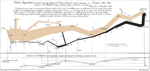
This flow map of Napoleon's ill-fated march on Moscow is an early and celebrated example of geovisualization. It shows the army's direction as it traveled, the places the troops passed through, the size of the army as troops died from hunger and wounds, and the freezing temperatures they experienced.

Geovisualization (GVis) combines scientific visualization with digital cartography to support the exploration and analysis of geographic data and information, including the results of spatial analysis or simulation. GVis leverages the human orientation towards visual information processing in the exploration, analysis and communication of geographic data and information. In contrast with traditional cartography, GVis is typically three or four-dimensional (the latter including time) and user-interactive.

Geographic knowledge discovery (GKD) is the human-centered process of applying efficient computational tools for exploring massive spatial databases. GKD includes geographic data mining, but also encompasses related activities such as data selection, data cleaning and pre-processing, and interpretation of results. GVis can also serve a central role in the GKD process. GKD is based on the premise that massive databases contain interesting (valid, novel, useful and understandable) patterns that standard analytical techniques cannot find. GKD can serve as a hypothesis-generating process for spatial analysis, producing tentative patterns and relationships that should be confirmed using spatial analytical techniques.

Spatial Decision Support Systems (sDSS) take existing spatial data and use a variety of mathematical models to make projections into the future. This allows urban and regional planners to test intervention decisions prior to implementation.

[edit] See also

• Complete spatial randomness
• Geodemographic segmentation
• Visibility analysis
• Suitability analysis
• Geospatial predictive modeling
• Geostatistics
• Extrapolation domain analysis
• Geoinformatics

[edit] References

1. ^ Mark Monmonier How to Lie with Maps University of Chicago Press, 1996.
2. ^ Tobler, W. (1970). A computer movie simulating urban growth in the Detroit region. Economic Geography, 46, 234-240.
3. ^ Longley and Batty Spatial Analysis: Modelling in a GIS Environment pp. 24-25
4. ^ Graham J. Upton & Bernard Fingelton: Spatial Data Analysis by Example Volume 1: Point Pattern and Quantitative Data John Wiley & Sons, New York. 1985.

[edit] Further reading

• Abler, R., J. Adams, and P. Gould (1971) Spatial Organization–The Geographer's View of the World, Englewood Cliffs, NJ: Prentice-Hall.
• Anselin, L. (1995) "Local indicators of spatial association – LISA". Geographical Analysis, 27, 93–115.
• Benenson, I. and P. M. Torrens. (2004). Geosimulation: Automata-Based Modeling of Urban Phenomena. Wiley.
• Fotheringham, A. S., C. Brunsdon and M. Charlton (2000) Quantitative Geography: Perspectives on Spatial Data Analysis, Sage.
• Fotheringham, A. S. and M. E. O'Kelly (1989) Spatial Interaction Models: Formulations and Applications, Kluwer Academic
• Fotheringham, A. S. and P. A. Rogerson (1993) "GIS and spatial analytical problems". International Journal of Geographical Information Systems, 7, 3–19.
• Goodchild, M. F. (1987) "A spatial analytical perspective on geographical information systems". International Journal of Geographical Information Systems, 1, 327–44.
• MacEachren, A. M. and D. R. F. Taylor (eds.) (1994) Visualization in Modern Cartography, Pergamon.
• Miller, H. J. (2004) "Tobler's First Law and spatial analysis". Annals of the Association of American Geographers, 94, 284–289.
• Miller, H. J. and J. Han (eds.) (2001) Geographic Data Mining and Knowledge Discovery, Taylor and Francis.
• O'Sullivan, D. and D. Unwin (2002) Geographic Information Analysis, Wiley.
• Parker, D. C., S. M. Manson, M.A. Janssen, M. J. Hoffmann and P. Deadman (2003) "Multi-agent systems for the simulation of land-use and land-cover change: A review". Annals of the Association of American Geographers, 93, 314–337.
• White, R. and G. Engelen (1997) "Cellular automata as the basis of integrated dynamic regional modelling". Environment and Planning B: Planning and Design, 24, 235–246.

[edit] External links

• ICA commission on geospatial analysis and modeling
• An educational resource about spatial statistics and geostatistics
• A comprehensive guide to principles, techniques & software tools
• Social and Spatial Inequalities
• National Center for Geographic Information and Analysis (NCGIA)

Scientific modelling

Jump to: navigation, search

This article may require cleanup to meet Wikipedia's quality standards. Please improve this article if you can. (February 2010)

Example of scientific modelling. A schematic of chemical and transport processes related to atmospheric composition.

Scientific modelling is the process of generating abstract, conceptual, graphical and/or mathematical models. Science offers a growing collection of methods, techniques and theory about all kinds of specialized scientific modelling. Also a way to read elements easily which have been broken down to the simplest form

Modelling is an essential and inseparable part of all scientific activity, and many scientific disciplines have their own ideas about specific types of modelling. There is little general theory about scientific modelling, offered by the philosophy of science, systems theory, and new fields like knowledge visualization.

Contents [hide] 1 Scientific modelling basics 1.1 Model 1.2 Modelling as a substitute for direct measurement and experimentation 1.3 Modelling language 1.4 Simulation 1.5 Structure 1.6 Systems 1.7 The process of generating a model 1.8 The process of evaluating a model 1.9 Visualization 2 Types of scientific modelling 2.1 Business process modelling 2.2 Other types 3 Applications 3.1 Modelling and Simulation 4 See also 5 References 6 Further reading 7 External links

[edit] Scientific modelling basics

[edit] Model

A model is a simplified abstract view of the complex reality. A scientific model represents empirical objects, phenomena, and physical processes in a logical way. Attempts to formalize the principles of the empirical sciences, use an interpretation to model reality, in the same way logicians axiomatize the principles of logic. The aim of these attempts is to construct a formal system for which reality is the only interpretation. The world is an interpretation (or model) of these sciences, only insofar as these sciences are true.^[1]

For the scientist, a model is also a way in which the human thought processes can be amplified.^[2] Models that are rendered in software allow scientists to leverage computational power to simulate, visualize, manipulate and gain intuition about the entity, phenomenon or process being represented.

[edit] Modelling as a substitute for direct measurement and experimentation

Models are typically used when it is either impossible or impractical to create experimental conditions in which scientists can directly measure outcomes. Direct measurement of outcomes under controlled conditions (see Controlled Experiment, Scientific Method) will always be more accurate than modeled estimates of outcomes. When predicting outcomes, models use assumptions, while measurements do not. As the number of assumptions in a model increases, the accuracy and relevance of the model diminishes.

[edit] Modelling language

A modelling language is any artificial language that can be used to express information or knowledge or systems in a structure that is defined by a consistent set of rules. The rules are used for interpretation of the meaning of components in the structure. Examples of modelling languages are the Unified Modeling Language (UML) for software systems, IDEF for processes and the VRML for 3-D computer graphics models designed particularly with the World Wide Web in mind.

[edit] Simulation

A simulation is the implementation of a model over time. A simulation brings a model to life and shows how a particular object or phenomenon will behave. It is useful for testing, analysis or training where real-world systems or concepts can be represented by a model.^[3]

[edit] Structure

Structure is a fundamental and sometimes intangible notion covering the recognition, observation, nature, and stability of patterns and relationships of entities. From a child's verbal description of a snowflake, to the detailed scientific analysis of the properties of magnetic fields, the concept of structure is an essential foundation of nearly every mode of inquiry and discovery in science, philosophy, and art.^[4]

[edit] Systems

A system is a set of interacting or interdependent entities, real or abstract, forming an integrated whole. The concept of an 'integrated whole' can also be stated in terms of a system embodying a set of relationships which are differentiated from relationships of the set to other elements, and from relationships between an element of the set and elements not a part of the relational regime.

[edit] The process of generating a model

Modelling refers to the process of generating a model as a conceptual representation of some phenomenon. Typically a model will refer only to some aspects of the phenomenon in question, and two models of the same phenomenon may be essentially different, that is in which the difference is more than just a simple renaming. This may be due to differing requirements of the model's end users or to conceptual or aesthetic differences by the modellers and decisions made during the modelling process. Aesthetic considerations that may influence the structure of a model might be the modeller's preference for a reduced ontology, preferences regarding probabilistic models vis-a-vis deterministic ones, discrete vs continuous time etc. For this reason users of a model need to understand the model's original purpose and the assumptions of its validity^{[citation needed]}.

[edit] The process of evaluating a model

A model is evaluated first and foremost by its consistency to empirical data; any model inconsistent with reproducible observations must be modified or rejected. However, a fit to empirical data alone is not sufficient for a model to be accepted as valid. Other factors important in evaluating a model include:^{[citation needed]}

• Ability to explain past observations
• Ability to predict future observations
• Cost of use, especially in combination with other models
• Refutability, enabling estimation of the degree of confidence in the model
• Simplicity, or even aesthetic appeal

People may attempt to quantify the evaluation of a model using a utility function.

[edit] Visualization

Visualization is any technique for creating images, diagrams, or animations to communicate a message. Visualization through visual imagery has been an effective way to communicate both abstract and concrete ideas since the dawn of man. Examples from history include cave paintings, Egyptian hieroglyphs, Greek geometry, and Leonardo da Vinci's revolutionary methods of technical drawing for engineering and scientific purposes.

[edit] Types of scientific modelling

[edit] Business process modelling

Abstraction for Business process modelling ^[5]

In business process modelling the enterprise process model is often referred to as the business process model. Process models are core concepts in the discipline of process engineering. Process models are:

• Processes of the same nature that are classified together into a model.
• A description of a process at the type level.
• Since the process model is at the type level, a process is an instantiation of it.

The same process model is used repeatedly for the development of many applications and thus, has many instantiations.

One possible use of a process model is to prescribe how things must/should/could be done in contrast to the process itself which is really what happens. A process model is roughly an anticipation of what the process will look like. What the process shall be will be determined during actual system development.^[6]

[edit] Other types

Analogical modelling Assembly modelling Catastrophe modelling Choice Modelling Climate model Continuous modelling Data modelling Document modelling Discrete modelling Economic model Ecosystem model

Empirical modelling Enterprise modelling Futures studies Geologic modelling Goal Modelling Homology modelling Hydrogeology Hydrography Hydrologic modelling Informative Modelling Mathematical modelling

Metabolic network modelling Modelling in Epidemiology Molecular modelling Modelling biological systems Multiscale modeling NLP modelling Predictive modelling Simulation Software modelling Solid modelling Statistics Stochastic modelling System dynamics

[edit] Applications

[edit] Modelling and Simulation

One application of scientific modelling is the field of "Modelling and Simulation", generally referred to as "M&S".^[7] M&S has a spectrum of applications which range from concept development and analysis, through experimentation, measurement and verification, to disposal analysis. Projects and programs may use hundreds of different simulations, simulators and model analysis tools.

Example of the integrated use of Modelling and Simulation in Defence life cycle management. The modelling and simulation in this image is represented in the center of the image with the three containers.^[3]

The figure shows how Modelling and Simulation is used as a central part of an integrated program in a Defence capability development process.^[3]

[edit] See also

• List of computer graphics and descriptive geometry topics
• List of graphical methods
• Modelling language
• Scientific visualization
• Seven Management and Planning Tools
• Simulation
• Systems Engineering
• Toy model

[edit] References

1. ^ edited by Hans Freudenthal (1951), The Concept and the Role of the Model in Mathematics and Natural and Social Sciences, p. 8-9
2. ^ C. West Churchman, The Systems Approach, New York: Dell publishing, 1968, p.61
3. ^ ^{a b c} Systems Engineering Fundamentals. Defense Acquisition University Press, 2003.
4. ^ Pullan, Wendy (2000). Structure. Cambridge: Cambridge University Press. ISBN 0521782589.
5. ^ Colette Rolland (1993). "Modeling the Requirements Engineering Process." in: 3rd European-Japanese Seminar on Information Modelling and Knowledge Bases, Budapest, Hungary, June 1993.
6. ^ C. Rolland and C. Thanos Pernici (1998). "A Comprehensive View of Process Engineering". In: Proceedings of the 10th International Conference CAiSE'98, B. Lecture Notes in Computer Science 1413, Pisa, Italy, Springer, June 1998.
7. ^ Because "Modeling and Simulation" is frequently taught in male dominated undergraduate environments, this field of application is deliberately named "Modeling and Simulation", rather than "Simulation and Modeling", to avoid distractions which may arise due to any possible association with the negative connotations of S&M.^{[citation needed]}

[edit] Further reading

Nowadays there are some 40 magazines about scientific modelling which offer all kinds of international forums. Since the 1960s there is a strong growing amount of books and magazines about specific forms of scientific modelling. There is also a lot of discussion about scientific modelling in the philosophy-of-science literature. A selection:

• C. West Churchman (1968). The Systems Approach, New York: Dell Publishing.
• Rainer Hegselmann, Ulrich Müller and Klaus Troitzsch (eds.) (1996). Modelling and Simulation in the Social Sciences from the Philosophy of Science Point of View. Theory and Decision Library. Dordrecht: Kluwer.
• Paul Humphreys (2004). Extending Ourselves: Computational Science, Empiricism, and Scientific Method. Oxford: Oxford University Press.
• Johannes Lenhard, Günter Küppers and Terry Shinn (Eds.) (2006) "Simulation: Pragmatic Constructions of Reality", Springer Berlin.
• Fritz Rohrlich (1990). "Computer Simulations in the Physical Sciences". In: Proceedings of the Philosophy of Science Association, Vol. 2, edited by Arthur Fine et al., 507-518. East Lansing: The Philosophy of Science Association.
• Rainer Schnell (1990). "Computersimulation und Theoriebildung in den Sozialwissenschaften". In: Kölner Zeitschrift für Soziologie und Sozialpsychologie 1, 109-128.
• Sergio Sismondo and Snait Gissis (eds.) (1999). Modeling and Simulation. Special Issue of Science in Context 12.
• Eric Winsberg (2001). "Simulations, Models and Theories: Complex Physical Systems and their Representations". In: Philosophy of Science 68 (Proceedings): 442-454.
• Eric Winsberg (2003). "Simulated Experiments: Methodology for a Virtual World". In: Philosophy of Science 70: 105–125.

Neuroimaging

Jump to: navigation, search

This article includes a list of references or external links, but its sources remain unclear because it has insufficient inline citations. Please help to improve this article by introducing more precise citations where appropriate. (April 2009)

Para-sagittal MRI of the head in a patient with benign familial macrocephaly.

3-D MRI of a section of the head.

Neuroimaging includes the use of various techniques to either directly or indirectly image the structure, function/pharmacology of the brain. It is a relatively new discipline within medicine and neuroscience/psychology.^[1]

Contents [hide] 1 Overview 2 History 3 Brain imaging techniques 3.1 Computed axial tomography 3.2 Diffuse optical imaging 3.3 Event-related optical signal 3.4 Magnetic resonance imaging 3.5 Functional magnetic resonance imaging 3.6 Electroencephalography 3.7 MagnetoEncephaloGraphy 3.8 Positron emission tomography 3.9 Single photon emission computed tomography 4 See also 5 References 6 Further reading 7 External links

[edit] Overview

Neuroimaging falls into two broad categories:

• Structural imaging, which deals with the structure of the brain and the diagnosis of gross (large scale) intracranial disease (such as tumor), and injury, and
• functional imaging, which is used to diagnose metabolic diseases and lesions on a finer scale (such as Alzheimer's disease) and also for neurological and cognitive psychology research and building brain-computer interfaces.

Functional imaging enables, for example, the processing of information by centers in the brain to be visualized directly. Such processing causes the involved area of the brain to increase metabolism and "light up" on the scan.

[edit] History

Main article: History of neuroimaging

In 1918 the American neurosurgeon Walter Dandy introduced the technique of ventriculography. X-ray images of the ventricular system within the brain were obtained by injection of filtered air directly into one or both lateral ventricles of the brain. Dandy also observed that air introduced into the subarachnoid space via lumbar spinal puncture could enter the cerebral ventricles and also demonstrate the cerebrospinal fluid compartments around the base of the brain and over its surface. This technique was called pneumoencephalography.

In 1927 Egas Moniz, professor of neurology in Lisbon and recipient of the Nobel Prize for Physiology or Medicine in 1949, introduced cerebral angiography, whereby both normal and abnormal blood vessels in and around the brain could be visualized with great accuracy.

In the early 1970s, Allan McLeod Cormack and Godfrey Newbold Hounsfield introduced computerized axial tomography (CAT or CT scanning), and ever more detailed anatomic images of the brain became available for diagnostic and research purposes. Cormack and Hounsfield won the 1979 Nobel Prize for Physiology or Medicine for their work. Soon after the introduction of CAT in the early 1980s, the development of radioligands allowed single photon emission computed tomography (SPECT) and positron emission tomography (PET) of the brain.

More or less concurrently, magnetic resonance imaging (MRI or MR scanning) was developed by researchers including Peter Mansfield and Paul Lauterbur, who were awarded the Nobel Prize for Physiology or Medicine in 2003. In the early 1980s MRI was introduced clinically, and during the 1980s a veritable explosion of technical refinements and diagnostic MR applications took place. Scientists soon learned that the large blood flow changes measured by PET could also be imaged by the correct type of MRI. Functional magnetic resonance imaging (fMRI) was born, and since the 1990s, fMRI has come to dominate the brain mapping field due to its low invasiveness, lack of radiation exposure, and relatively wide availability. As noted above fMRI is also beginning to dominate the field of stroke treatment.

In early 2000s the field of neuroimaging reached the stage where limited practical applications of functional brain imaging have become feasible. The main application area is crude forms of brain-computer interface.

[edit] Brain imaging techniques

[edit] Computed axial tomography

Computed tomography (CT) or Computed Axial Tomography (CAT) scanning uses a series of x-rays of the head taken from many different directions. Typically used for quickly viewing brain injuries, CT scanning uses a computer program that performs a numerical integral calculation (the inverse Radon transform) on the measured x-ray series to estimate how much of an x-ray beam is absorbed in a small volume of the brain. Typically the information is presented as cross sections of the brain.^[2]

In approximation, the denser a material is, the whiter a volume of it will appear on the scan (just as in the more familiar "flat" X-rays). CT scans are primarily used for evaluating swelling from tissue damage in the brain and in assessment of ventricle size. Modern CT scanning can provide reasonably good images in a matter of minutes.

[edit] Diffuse optical imaging

Diffuse optical imaging (DOI) or diffuse optical tomography (DOT) is a medical imaging modality which uses near infrared light to generate images of the body. The technique measures the optical absorption of haemoglobin, and relies on the absorption spectrum of haemoglobin varying with its oxygenation status.

[edit] Event-related optical signal

Event-related optical signal (EROS) is a brain-scanning technique which uses infrared light through optical fibers to measure changes in optical properties of active areas of the cerebral cortex. Whereas techniques such as diffuse optical imaging (DOT) and near infrared spectroscopy (NIRS) measure optical absorption of haemoglobin, and thus are based on blood flow, EROS takes advantage of the scattering properties of the neurons themselves, and thus provides a much more direct measure of cellular activity. EROS can pinpoint activity in the brain within millimeters (spatially) and within milliseconds (temporally). Its biggest downside is the inability to detect activity more than a few centimeters deep. EROS is a new, relatively inexpensive technique that is non-invasive to the test subject. It was developed at the University of Illinois at Urbana-Champaign where it is now used in the Cognitive Neuroimaging Laboratory of Dr. Gabriele Gratton and Dr. Monica Fabiani.

[edit] Magnetic resonance imaging

Sagittal MRI slice at the midline.

Magnetic resonance imaging (MRI) uses magnetic fields and radio waves to produce high quality two- or three-dimensional images of brain structures without use of ionizing radiation (X-rays) or radioactive tracers. During an MRI, a large cylindrical magnet creates a magnetic field around the head of the patient through which radio waves are sent. When the magnetic field is imposed, each point in space has a unique radio frequency at which the signal is received and transmitted (Preuss). Sensors read the frequencies and a computer uses the information to construct an image. The detection mechanisms are so precise that changes in structures over time can be detected.^[1]

Using MRI, scientists can create images of both surface and subsurface structures with a high degree of anatomical detail. MRI scans can produce cross sectional images in any direction from top to bottom, side to side, or front to back. The problem with original MRI technology was that while it provides a detailed assessment of the physical appearance, water content, and many kinds of subtle derangements of structure of the brain (such as inflammation or bleeding), it fails to provide information about the metabolism of the brain (i.e. how actively it is functioning) at the time of imaging. A distinction is therefore made between "MRI imaging" and "functional MRI imaging" (fMRI), where MRI provides only structural information on the brain while fMRI yields both structural and functional data.

[edit] Functional magnetic resonance imaging

Axial MRI slice at the level of the basal ganglia, showing fMRI BOLD signal changes overlayed in red (increase) and blue (decrease) tones.

Functional magnetic resonance imaging (fMRI) relies on the paramagnetic properties of oxygenated and deoxygenated hemoglobin to see images of changing blood flow in the brain associated with neural activity. This allows images to be generated that reflect which brain structures are activated (and how) during performance of different tasks.

Most fMRI scanners allow subjects to be presented with different visual images, sounds and touch stimuli, and to make different actions such as pressing a button or moving a joystick. Consequently, fMRI can be used to reveal brain structures and processes associated with perception, thought and action. The resolution of fMRI is about 2-3 millimeters at present, limited by the spatial spread of the hemodynamic response to neural activity. It has largely superseded PET for the study of brain activation patterns. PET, however, retains the significant advantage of being able to identify specific brain receptors (or transporters) associated with particular neurotransmitters through its ability to image radiolabelled receptor "ligands" (receptor ligands are any chemicals that stick to receptors).

As well as research on healthy subjects, fMRI is increasingly used for the medical diagnosis of disease. Because fMRI is exquisitely sensitive to blood flow, it is extremely sensitive to early changes in the brain resulting from ischemia (abnormally low blood flow), such as the changes which follow stroke. Early diagnosis of certain types of stroke is increasingly important in neurology, since substances which dissolve blood clots may be used in the first few hours after certain types of stroke occur, but are dangerous to use afterwards. Brain changes seen on fMRI may help to make the decision to treat with these agents. With between 72% and 90% accuracy where chance would achieve 0.8%,^[3] fMRI techniques can decide which of a set of known images the subject is viewing.^[4]

[edit] Electroencephalography

Electroencephalography (EEG) is an imaging technique used to measure the electric fields in the brain via electrodes placed on the scalp of a human. EEG offers a very direct measurement of neural electrical activity with very high temporal resolution but relatively low spatial resolution. ^[5]

[edit] MagnetoEncephaloGraphy

Magnetoencephalography (MEG) is an imaging technique used to measure the magnetic fields produced by electrical activity in the brain via extremely sensitive devices such as superconducting quantum interference devices (SQUIDs). MEG offers a very direct measurement neural electrical activity (compared to fMRI for example) with very high temporal resolution but relatively low spatial resolution. The advantage of measuring the magnetic fields produced by neural activity is that they are not distorted by surrounding tissue, unlike the electric fields measured by EEG (particularly the skull and scalp).

There are many uses for the MEG, including assisting surgeons in localizing a pathology, assisting researchers in determining the function of various parts of the brain, neurofeedback, and others.

[edit] Positron emission tomography

PET scan of a normal 20-year-old brain.

Positron emission tomography (PET) measures emissions from radioactively labeled metabolically active chemicals that have been injected into the bloodstream. The emission data are computer-processed to produce 2- or 3-dimensional images of the distribution of the chemicals throughout the brain. ^[6] The positron emitting radioisotopes used are produced by a cyclotron, and chemicals are labeled with these radioactive atoms. The labeled compound, called a radiotracer, is injected into the bloodstream and eventually makes its way to the brain. Sensors in the PET scanner detect the radioactivity as the compound accumulates in various regions of the brain. A computer uses the data gathered by the sensors to create multicolored 2- or 3-dimensional images that show where the compound acts in the brain. Especially useful are a wide array of ligands used to map different aspects of neurotransmitter activity, with by far the most commonly used PET tracer being a labeled form of glucose (see FDG).

The greatest benefit of PET scanning is that different compounds can show blood flow and oxygen and glucose metabolism in the tissues of the working brain. These measurements reflect the amount of brain activity in the various regions of the brain and allow to learn more about how the brain works. PET scans were superior to all other metabolic imaging methods in terms of resolution and speed of completion (as little as 30 seconds), when they first became available. The improved resolution permitted better study to be made as to the area of the brain activated by a particular task. The biggest drawback of PET scanning is that because the radioactivity decays rapidly, it is limited to monitoring short tasks. ^[7] Before fMRI technology came online, PET scanning was the preferred method of functional (as opposed to structural) brain imaging, and it still continues to make large contributions to neuroscience.

PET scanning is also used for diagnosis of brain disease, most notably because brain tumors, strokes, and neuron-damaging diseases which cause dementia (such as Alzheimer's disease) all cause great changes in brain metabolism, which in turn causes easily detectable changes in PET scans. PET is probably most useful in early cases of certain dementias (with classic examples being Alzheimer's disease and Pick's disease) where the early damage is too diffuse and makes too little difference in brain volume and gross structure to change CT and standard MRI images enough to be able to reliably differentiate it from the "normal" range of cortical atrophy which occurs with aging (in many but not all) persons, and which does not cause clinical dementia.

[edit] Single photon emission computed tomography

Single photon emission computed tomography (SPECT) is similar to PET and uses gamma ray emitting radioisotopes and a gamma camera to record data that a computer uses to construct two- or three-dimensional images of active brain regions^[8] SPECT relies on an injection of radioactive tracer, which is rapidly taken up by the brain but does not redistribute. Uptake of SPECT agent is nearly 100% complete within 30 – 60s, reflecting cerebral blood flow (CBF) at the time of injection. These properties of SPECT make it particularly well suited for epilepsy imaging, which is usually made difficult by problems with patient movement and variable seizure types. SPECT provides a "snapshot" of cerebral blood flow since scans can be acquired after seizure termination (so long as the radioactive tracer was injected at the time of the seizure). A significant limitation of SPECT is its poor resolution (about 1 cm) compared to that of MRI.

Like PET, SPECT also can be used to differentiate different kinds of disease processes which produce dementia, and it is increasingly used for this purpose. Neuro-PET has a disadvantage of requiring use of tracers with half-lives of at most 110 minutes, such as FDG. These must be made in a cyclotron, and are expensive or even unavailable if necessary transport times are prolonged more than a few half-lives. SPECT, however, is able to make use of tracers with much longer half-lives, such as technetium-99m, and as a result, is far more widely available.

[edit] See also

• Brain mapping
• Functional neuroimaging
• functional near-infrared imaging
• History of brain imaging
• Human Cognome Project
• Magnetic resonance imaging
• Magnetoencephalography
• Medical imaging
• Neuroimaging software
• Statistical parametric mapping
• Transcranial magnetic stimulation
• Voxel-based morphometry

[edit] References

1. ^ ^{a b} Filler, AG: The history, development, and impact of computed imaging in neurological diagnosis and neurosurgery: CT, MRI, DTI: Nature Precedings DOI: 10.1038/npre.2009.3267.5.Neurosurgical Focus (in press)
2. ^ Jeeves, p. 21
3. ^ Smith, Kerri (March 5, 2008). "Mind-reading with a brain scan". Nature News (Nature Publishing Group). http://www.nature.com/news/2008/080305/full/news.2008.650.html. Retrieved 2008-03-05.
4. ^ Keim, Brandon (March 5, 2008). "Brain Scanner Can Tell What You're Looking At". Wired News (CondéNet). http://www.wired.com/science/discoveries/news/2008/03/mri_vision. Retrieved 2008-03-05.
5. ^ Berger, H. (1929). Über das Elektroenkephalogramm des Menschen. European Archives of Psychiatry and Clinical Neuroscience. 87(1), 527:570.
6. ^ Nilsson, page 57
7. ^ Nilson, pg. 60
8. ^ Philip Ball Brain Imaging Explained

[edit] Further reading

• Philip Ball. Brain Imaging Explained.
• J. Graham Beaumont (1983). Introduction to Neuropsychology. New York: The Guilford Press.
• Jean-Pierre Changeux (1985). Neuronal Man: The Biology of Mind. New York: Oxford University Press.
• Malcom Jeeves (1994). Mind Fields: Reflections on the Science of Mind and Brain. Grand Rapids, MI: Baker Books.
• Richard G. Lister and Herbert J. Weingartner (1991). Perspectives on Cognitive Neuroscience. New York: Oxford University Press.
• James Mattson and Merrill Simon (1996). The Pioneers of NMR and Magnetic Resonance in Medicine. United States: Dean Books Company.
• Lars-Goran Nilsson and Hans J. Markowitsch (1999). Cognitive Neuroscience of Memory. Seattle: Hogrefe & Huber Publishers.
• Donald A. Norman (1981). Perspectives on Cognitive Science. New Jersey: Ablex Publishing Corporation.
• Brenda Rapp (2001). The Handbook of Cognitive Neuropsychology. Ann Arbor, MI: Psychology Press.
• Berger, H. (1929). Über das Elektroenkephalogramm des Menschen. European Archives of Psychiatry and Clinical Neuroscience. 87(1), 527:570.